INTRODUCTION
Cancer detection is one of the most critical areas where machine learning can make a real difference. This project focused on using two methods of machine learning to predict whether a patient's tumor as seen in an MRI scan was malignant or benign. We built a Convolutional Neural Network from scratch in Python, and created Bayesian Logistic Regression Models using packages in R.
DATA PREPARATION & CLEANING
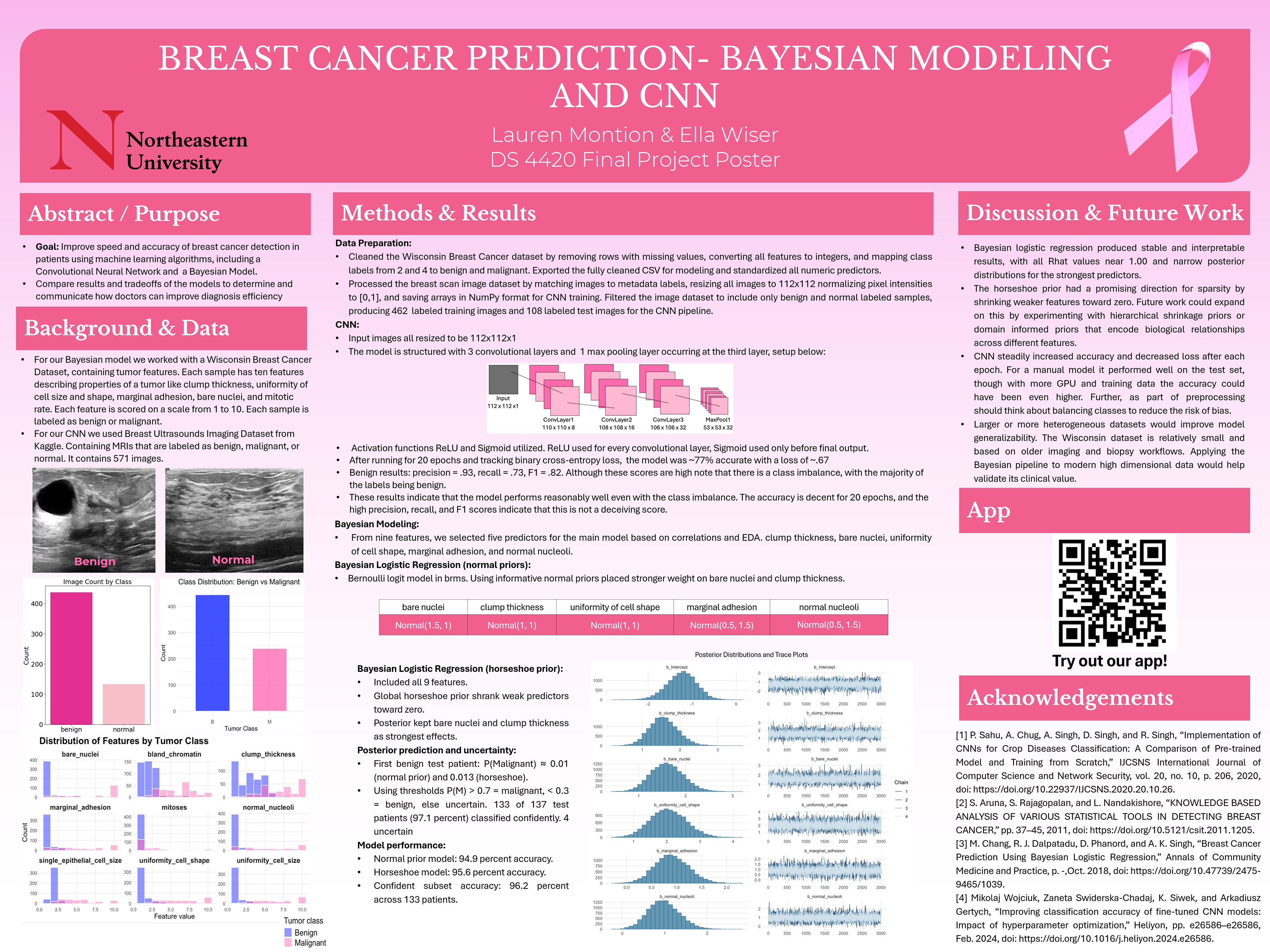
The CNN used the Dataset_BUSI_with_GT image dataset from Kaggle, containing ultrasound scans labeled as benign, malignant, or normal. After an initial attempt at classifying malignancy proved infeasible (accuracy below 50%), the problem was reframed as detecting whether a tumor was benign or not, leaving 462 training images and 108 test images. Images were loaded at 112x112 pixels, converted to NumPy arrays, and standardized. The Bayesian models used the Wisconsin Breast Cancer Diagnostic dataset, which contains nine cell morphology features extracted from fine needle aspirate samples. All features were standardized and split 80/20 into training and test sets.
CONVOLUTIONAL NEURAL NETWORK (CNN) IN PYTHON
To build a CNN from scratch, five classes were created in Python to cover each component: ConvLayers, MaxPool, FullyConnect, ReLU, and Sigmoid. Additionally, a binary cross-entropy loss and its derivative for backpropagation were defined for training. The architecture uses three convolutional layers with ReLU activations, a max pooling layer, and two fully connected layers ending in a sigmoid output. Training used a batch size of 16 and ran for 20 epochs at a learning rate of 0.005, with data shuffled each epoch to prevent order-dependent learning. The final model achieved 77.7% accuracy on the test set with a precision of 0.931 and an F1 score of 0.818, promising results given the small training set and the computational constraints of running each epoch locally. Note that due to long training times and lack of computer power, more epochs could not be run.
BAYESIAN LOGISTIC REGRESSION IN R
Three Bayesian models were built in R using the brms package, each adding complexity to understand how the framework scales. The first used the bare nuclei characteristic as a single predictor, which alone reached 94% accuracy and showed a posterior coefficient distribution clearly separated from zero. The second expanded to five predictors with informative Normal priors, achieving 94.9% accuracy and a ROC AUC of 0.992. The third applied a horseshoe prior across all nine features, allowing the model to automatically shrink weaker predictors. Mitoses and single epithelial cell size faded out while clump thickness, bare nuclei, and uniformity of cell shape remained dominant. This model reached 95.6% accuracy. A key highlight was applying a cost-sensitive classification threshold: since missing a malignant tumor is far more dangerous than a false positive, false negatives were weighted 10x more than false positives. This shifted the optimal threshold from 0.50 to 0.08, boosting accuracy to 96.4% with perfect sensitivity on the test set.